Products: Abaqus/Standard Abaqus/Explicit
Several methods of specifying time variations of prescribed magnitudes are tested through the use of the amplitude curve.
The amplitude curve is used to specify a function that defines arbitrary time variations of prescribed variables throughout an analysis. The user can specify this function with a variety of methods. Two of the methods use tabulated values that define a continuous function of linear segments. The tabular amplitude definition uses a nonfixed time increment, which requires that pairs of time-amplitude data be supplied. The equally spaced amplitude definition uses a fixed time increment that is specified once, and only the values of the function are required. Two other amplitude types use trigonometric functions to define the function. The periodic amplitude definition uses the Fourier series to define the function. The modulated amplitude definition uses the product of two sine functions. The exponential decay amplitude definition uses an exponential function. The smooth-step amplitude definition uses a fifth-order polynomial equation to ramp up/down smoothly from one amplitude value to the next. A solution-dependent amplitude definition (available only in Abaqus/Standard) accepts a starting value and lets Abaqus calculate subsequent values based on the evolution of solution parameters. Currently there is only one solution parameter available, the maximum equivalent creep strain rate, which is compared to target values entered in the creep strain rate.
If the function describes either a displacement or velocity in a dynamic analysis, the derivatives and integrations of the function are required. For the three amplitude types that use trigonometric or exponential functions, the derivatives are continuous and available. For the amplitude type that uses a fifth-order polynomial equation, the derivatives are continuous and available; however, both the first and second derivatives are zero at the data point. For the two types that use tabulated values, the linear segments do not have continuous derivatives, and the second derivative will be infinite at the segment intersections. An amplitude curve with smoothing allows the user to define an interval about the data points in which a quadratic function is interpolated to give a continuous first derivative and a finite second derivative. The use of this parameter is verified within these tests.
Input files xampmult.inp (Abaqus/Standard) and xamptest.inp (Abaqus/Explicit) are analyses performed over multiple steps during which several loads and displacements are applied in terms of defined amplitudes with various settings of the parameters. xampresm.inp (Abaqus/Standard) and xamprest.inp (Abaqus/Explicit) restart the analyses from the previous step. A simple truss model is used. Various nodal degrees of freedom are prescribed with the boundary conditions, and loads are applied. In all of these cases the prescribed quantities are defined using the amplitude curve. The purpose of this test is to ensure that the initial value of the function to be applied in the next step is interpolated properly from the amplitude definitions. Since xampresm.inp and xamprest.inp restart the analysis from the previous step, the results will show that the initial value at the beginning of the restart step is obtained from the point on the amplitude curve at which the restart was done; the value will be ramped to the new value defined in the new step. The output variables corresponding to the prescribed input are checked to verify the use of the amplitude curve.
xampsdep.inp and xampress.inp simulate the superplastic forming of a rectangular pan in Abaqus/Standard. The pressure applied to a sheet that forces it to acquire the shape of a die is determined by solution-dependent amplitude.
The results for each of the amplitude types are discussed in the following sections.
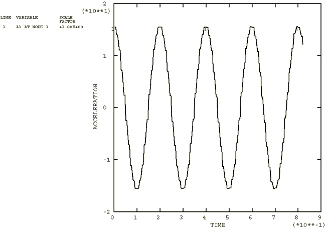
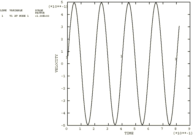
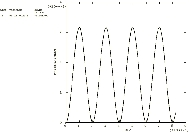
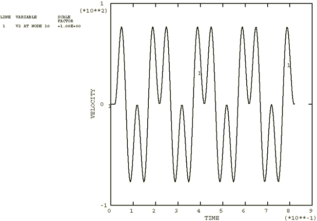
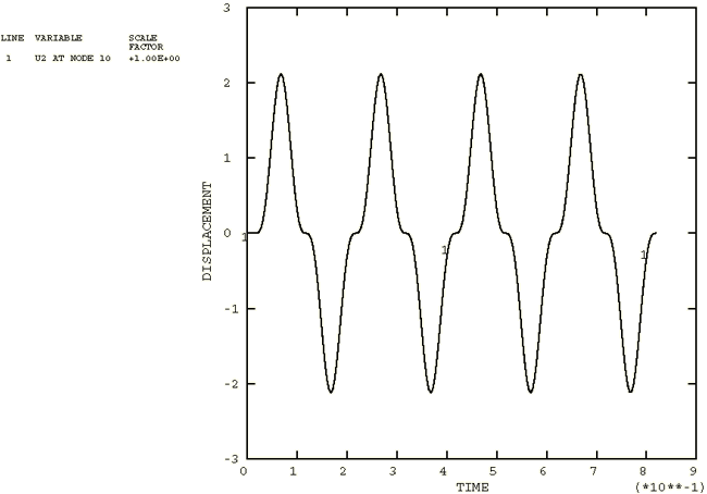
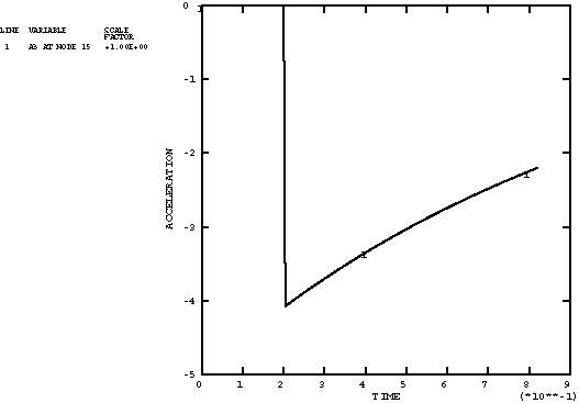
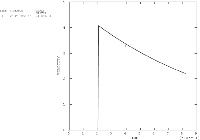
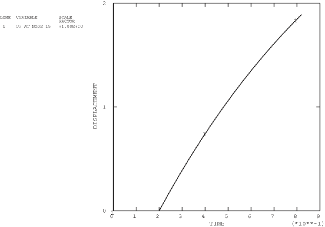
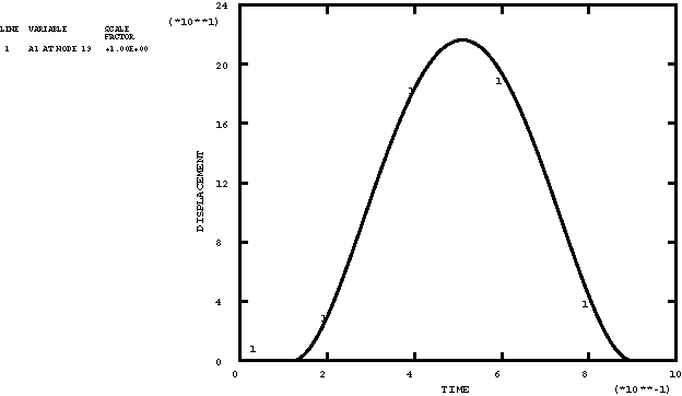
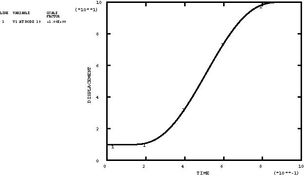
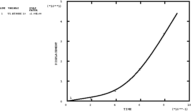
A typical variation of a boundary condition is shown in the history plots of Figure 5.1.3–1 through Figure 5.1.3–3. For this particular example of the variation, the velocity history is specified. The tabulated input is given to represent a sine curve. The acceleration history shown is the time derivative of the velocity curve. The displacement history is the integration of the velocity curve. Various other types of boundary conditions and specified curves are verified in the test.
One of the boundary condition variations used in xampmult.inp and xamptest.inp is specified with the velocity history. The variation is specified using a sinusoidal variation corresponding to the following expression: ![]() . This variation was chosen such that it is identical to the function specified using tabulated values in the previous section. The acceleration, velocity, and displacement histories are the same as those from the previous section, as shown in Figure 5.1.3–1 through Figure 5.1.3–3.
. This variation was chosen such that it is identical to the function specified using tabulated values in the previous section. The acceleration, velocity, and displacement histories are the same as those from the previous section, as shown in Figure 5.1.3–1 through Figure 5.1.3–3.
The velocity history is specified in xampmult.inp and xamptest.inp. This particular variation is specified using a fixed time step. The variation was chosen such that it is identical to the function specified using tabulated values without fixed time steps (see Tabular amplitude definition). The acceleration, velocity, and displacement histories are the same as those discussed previously and are shown in Figure 5.1.3–1 through Figure 5.1.3–3.
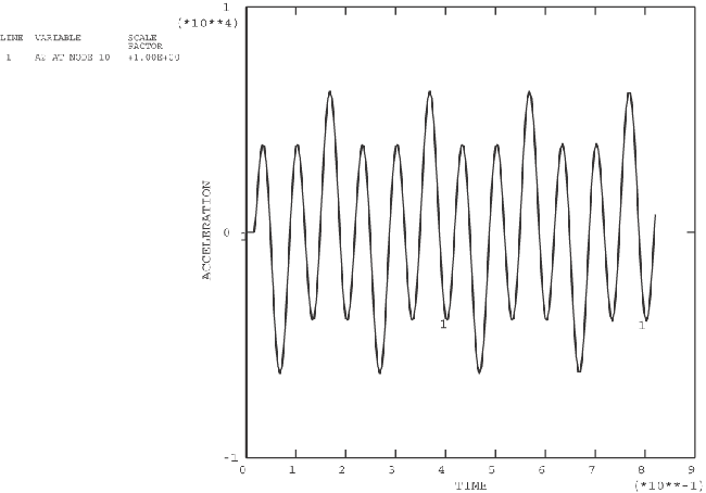
One of the boundary condition variations used in xampmult.inp and xamptest.inp is specified with the velocity history using a scale factor of 100.0. The variation is specified using a combination of sinusoidal functions corresponding to the following expression:
![]()
One of the boundary condition variations used in xampmult.inp and xamptest.inp is specified with the velocity history using a scale factor of 200. The variation is specified using an exponential function corresponding to the following expression:
![]()
One of the boundary condition variations used in xampmult.inp and xamptest.inp is specified with the velocity history using a scale factor of 100.0. The variation is specified using a polynomial equation corresponding to the following expression:
![]()
![]()
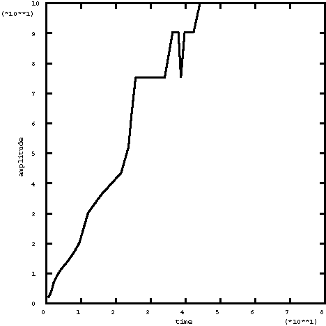
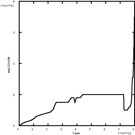
The initial value of the pressure is 1.0, and the amplitude is allowed to increase to 100 times that value (as well as decrease to 0.1 times the initial value). The maximum amplitude was reached, and Abaqus/Standard stopped the analysis because it could not follow the objective within the restrictions imposed. This happened before the sheet completely filled the die cavity. A restart run, xampress.inp, in which the maximum amplitude is modified to 500 times the reference load allows the deformation to be completed. Once again, the maximum allowable amplitude is used as the mechanism for Abaqus/Standard to end the analysis. The restart run exemplifies another possibility that is generally not recommended (since it will probably not occur in practice)—the loading reference value was increased by a factor of 5.0. As a result, the amplitude history adapted itself accordingly.
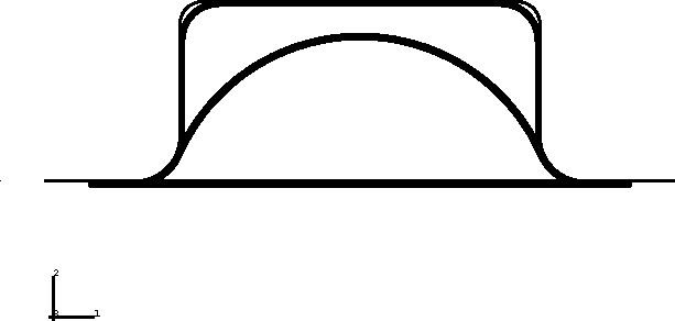
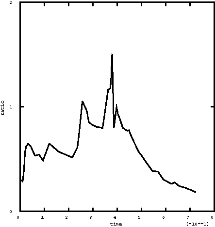
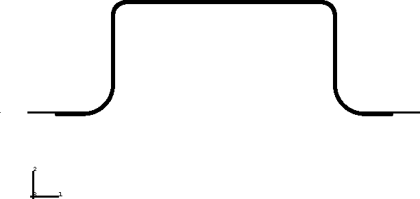
Figure 5.1.3–13 and Figure 5.1.3–16 show the rigid surface and the deformable sheet at different stages of deformation. Figure 5.1.3–14 and Figure 5.1.3–17 show the amplitude history obtained. Figure 5.1.3–15 shows the ratio between the maximum creep strain rate in the model and the target value provided.
*AMPLITUDE used over multiple steps.
*RESTART test of xampmult.inp.
*AMPLITUDE,DEFINITION=SOLUTION DEPENDENT.
*RESTART test of xampsdep.inp.
*AMPLITUDE used over multiple steps.
*RESTART test of xamptest.inp.