Product: Abaqus/Standard
This section provides basic verification tests for the fluid pipe and fluid pipe connector elements, which are used to model fluid flow in a pipe in Abaqus/Standard.
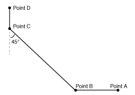
Fluid pipe elements are used to model the flow of fluid in a wellbore, as shown in Figure 1.3.41–1. The well consists of a vertical, a horizontal, and a deviated section. The deviated section is connected to the horizontal and vertical sections by fluid pipe connector elements. Two scenarios of laminar and turbulent flows are modeled in the wellbore. Point A is located 2000 m below ground level, and point D is located at ground level. The lengths of the horizontal and vertical sections are 1000 m and 500 m, respectively. The diameter of the pipe is 0.1 m. The connectors are modeled as two elbow joints. The connector loss coefficient used in this model is 0.64.
Material:
The fluid is modeled as an incompressible liquid with a density of 1000 kg/m3 and viscosity of 0.001 Pa∙sec.
Loading:
For laminar flow an inlet fluid flow rate of 12.4 × 10³ m3/s at point D and a pressure of 34.47 MPa at point A are prescribed. For turbulent flow an inlet flow rate of 10.77 × 10³ m3/s at point D and a pressure of 53.1 MPa at point A are specified.
Since the fluid is incompressible, the pressures can be computed using the Bernoulli equation for pipe flow.
The analytical pressures computed using the Bernoulli equation for pipe flow at points A to D are shown in the table below. Since the prescribed boundary conditions for the laminar and turbulent flows are different, the computed pressures are different for the two cases. The computed pressures for the laminar and turbulent flows in the deviated wellbore match the analytical solution.
FP2D2 and FPC2D2 elements with laminar flow.
FP3D2 and FPC3D2 elements with laminar flow.
FP2D2 and FPC2D2 elements with turbulent flow.
FP3D2 and FPC3D2 elements with turbulent flow.