Products: Abaqus/Explicit Abaqus/CAE
Equations of state:
provide a hydrodynamic material model in which the material's volumetric strength is determined by an equation of state;
determine the pressure (positive in compression) as a function of the density, ![]() , and the specific energy (the internal energy per unit mass),
, and the specific energy (the internal energy per unit mass), ![]() :
: ![]() ;
;
are available as Mie-Grüneisen equations of state (thus providing the linear ![]() Hugoniot form);
Hugoniot form);
are available as tabulated equations of state linear in energy;
are available as ![]() equations of state for the compaction of ductile porous materials and must be used in conjunction with either the Mie-Grüneisen or the tabulated equation of state for the solid phase;
equations of state for the compaction of ductile porous materials and must be used in conjunction with either the Mie-Grüneisen or the tabulated equation of state for the solid phase;
are available as JWL high explosive equations of state;
are available as ignition and growth equations of state;
are available in the form of an ideal gas;
are available in the form of user-defined equations of state (VUEOS);
assume an adiabatic condition unless a dynamic fully coupled temperature-displacement analysis is used;
can be used to model a material that has only volumetric strength (the material is assumed to have no shear strength) or a material that also has isotropic elastic or viscous deviatoric behavior;
can be used with the Mises (“Classical metal plasticity,” Section 23.2.1) or the Johnson-Cook (“Johnson-Cook plasticity,” Section 23.2.7) plasticity models;
can be used with the extended Drucker-Prager (“Extended Drucker-Prager models,” Section 23.3.1) plasticity models (without plastic dilation); and
can be used with the tensile failure model (“Dynamic failure models,” Section 23.2.8) to model dynamic spall or a pressure cutoff.
The equation for conservation of energy equates the increase in internal energy per unit mass, ![]() , to the rate at which work is being done by the stresses and the rate at which heat is being added. In the absence of heat conduction the energy equation can be written as
, to the rate at which work is being done by the stresses and the rate at which heat is being added. In the absence of heat conduction the energy equation can be written as
![]()
The equation of state is assumed for the pressure as a function of the current density, ![]() , and the internal energy per unit mass,
, and the internal energy per unit mass, ![]() :
:
![]()
An equation of state is said to be linear in energy when it can be written in the form
![]()
A Mie-Grüneisen equation of state is linear in energy. The most common form is
![]()
![]()
The Hugoniot energy, ![]() , is related to the Hugoniot pressure by
, is related to the Hugoniot pressure by
![]()
![]()
The equation of state and the energy equation represent coupled equations for pressure and internal energy. Abaqus/Explicit solves these equations simultaneously at each material point.
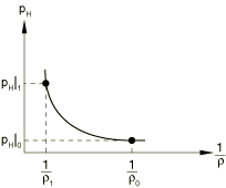
A common fit to the Hugoniot data is given by
![]()
![]()
![]()
There is a limiting compression given by the denominator of this form of the equation of state
![]()
![]()
| Abaqus/CAE Usage: | Property module: material editor:
General |
The initial state of the material is determined by the initial values of specific energy, ![]() , and pressure stress, p. Abaqus/Explicit will automatically compute the initial density,
, and pressure stress, p. Abaqus/Explicit will automatically compute the initial density, ![]() , that satisfies the equation of state,
, that satisfies the equation of state, ![]() . You can define the initial specific energy and initial stress state (see “Initial conditions in Abaqus/Standard and Abaqus/Explicit,” Section 34.2.1). The initial pressure used by the equation of state is inferred from the specified stress states. If no initial conditions are specified, Abaqus/Explicit will assume that the material is at its reference state:
. You can define the initial specific energy and initial stress state (see “Initial conditions in Abaqus/Standard and Abaqus/Explicit,” Section 34.2.1). The initial pressure used by the equation of state is inferred from the specified stress states. If no initial conditions are specified, Abaqus/Explicit will assume that the material is at its reference state:

| Input File Usage: | Use either or both of the following options, as required: |
*INITIAL CONDITIONS, TYPE=SPECIFIC ENERGY *INITIAL CONDITIONS, TYPE=STRESS |
| Abaqus/CAE Usage: | Load module: Create Predefined Field: Step: Initial: choose Mechanical for the Category and Stress for the Types for Selected Step |
Initial specific energy is not supported in Abaqus/CAE. |
The tabulated equation of state provides flexibility in modeling the hydrodynamic response of materials that exhibit sharp transitions in the pressure-density relationship, such as those induced by phase transformations. The tabulated equation of state is linear in energy and assumes the form
![]()
You can specify the functions ![]() and
and ![]() directly in tabular form. The tabular entries must be given in descending values of the volumetric strain (that is, from the most tensile to the most compressive states). Abaqus/Explicit will use a piecewise linear relationship between data points. Outside the range of specified values of volumetric strains, the functions are extrapolated based on the last slope computed from the data.
directly in tabular form. The tabular entries must be given in descending values of the volumetric strain (that is, from the most tensile to the most compressive states). Abaqus/Explicit will use a piecewise linear relationship between data points. Outside the range of specified values of volumetric strains, the functions are extrapolated based on the last slope computed from the data.
| Abaqus/CAE Usage: | Property module: material editor:
General |
The initial state of the material is determined by the initial values of specific energy, ![]() , and pressure stress, p. Abaqus/Explicit automatically computes the initial density,
, and pressure stress, p. Abaqus/Explicit automatically computes the initial density, ![]() , that satisfies the equation of state. You can define the initial specific energy and initial stress state (see “Initial conditions in Abaqus/Standard and Abaqus/Explicit,” Section 34.2.1). The initial pressure used by the equation of state is inferred from the specified stress states. If no initial conditions are specified, Abaqus/Explicit assumes that the material is at its reference state:
, that satisfies the equation of state. You can define the initial specific energy and initial stress state (see “Initial conditions in Abaqus/Standard and Abaqus/Explicit,” Section 34.2.1). The initial pressure used by the equation of state is inferred from the specified stress states. If no initial conditions are specified, Abaqus/Explicit assumes that the material is at its reference state:
| Input File Usage: | Use either or both of the following options, as required: |
*INITIAL CONDITIONS, TYPE=SPECIFIC ENERGY *INITIAL CONDITIONS, TYPE=STRESS |
| Abaqus/CAE Usage: | Load module: Create Predefined Field: Step: Initial: choose Mechanical for the Category and Stress for the Types for Selected Step |
Initial specific energy is not supported in Abaqus/CAE. |
The user-defined equation of state provides a general capability for modeling the volumetric response of materials through user subroutine VUEOS (see “VUEOS,” Section 1.2.15 of the Abaqus User Subroutines Reference Guide). The equation of state defines the pressure as a function of the current density, ![]() , and the internal energy per unit mass,
, and the internal energy per unit mass, ![]() :
: ![]() . Abaqus/Explicit solves the energy equation together with the equation of state using an iterative method. The pressure stress,
. Abaqus/Explicit solves the energy equation together with the equation of state using an iterative method. The pressure stress, ![]() , and the derivatives of the pressure with respect to the internal energy and to the density,
, and the derivatives of the pressure with respect to the internal energy and to the density, ![]() and
and ![]() , must be provided by user subroutine VUEOS. The latter is needed for the evaluation of the effective bulk modulus of the material, which is necessary for the stable time increment calculation.
, must be provided by user subroutine VUEOS. The latter is needed for the evaluation of the effective bulk modulus of the material, which is necessary for the stable time increment calculation.
Optionally, you can also specify the number of property values needed as data in the user subroutine as well as the number of solution-dependent variables (see “User subroutines: overview,” Section 18.1.1).
| Input File Usage: | Use the following option: |
*EOS, TYPE=USER, PROPERTIES=n |
| Abaqus/CAE Usage: | The user-defined equation of state is not supported in Abaqus/CAE. |
You need to make sure that the initial specific energy, the initial stress, and the initial density satisfy the equation of state. If you do not specify the initial conditions, Abaqus/Explicit assumes that the material is at its reference state:
| Input File Usage: | Use either or both of the following options to define the initial specific energy and/or initial pressure stress: |
*INITIAL CONDITIONS, TYPE=SPECIFIC ENERGY
*INITIAL CONDITIONS, TYPE=STRESS
Use the following option to define the initial density: *DENSITY |
| Abaqus/CAE Usage: | Load module: Create Predefined Field: Step: Initial: choose Mechanical for the Category and Stress for the Types for Selected Step |
Initial specific energy is not supported in Abaqus/CAE. |
The ![]() equation of state is designed for modeling the compaction of ductile porous materials. The implementation in Abaqus/Explicit is based on the model proposed by Hermann (1968) and Carroll and Holt (1972). The constitutive model provides a detailed description of the irreversible compaction behavior at low stresses and predicts the correct thermodynamic behavior at high pressures for the fully compacted solid material. In Abaqus/Explicit the solid phase is assumed to be governed by either the Mie-Grüneisen equation of state or the tabulated equation of state. The relevant properties of the porous material in the virgin state, to be discussed later, and the material properties of the solid phase are specified separately.
equation of state is designed for modeling the compaction of ductile porous materials. The implementation in Abaqus/Explicit is based on the model proposed by Hermann (1968) and Carroll and Holt (1972). The constitutive model provides a detailed description of the irreversible compaction behavior at low stresses and predicts the correct thermodynamic behavior at high pressures for the fully compacted solid material. In Abaqus/Explicit the solid phase is assumed to be governed by either the Mie-Grüneisen equation of state or the tabulated equation of state. The relevant properties of the porous material in the virgin state, to be discussed later, and the material properties of the solid phase are specified separately.
The porosity of the material, n, is defined as the ratio of pore volume, ![]() , to total volume,
, to total volume, ![]() , where
, where ![]() is the solid volume. The porosity remains in the range
is the solid volume. The porosity remains in the range ![]() , with 0 indicating full compaction. It is convenient to introduce a scalar variable
, with 0 indicating full compaction. It is convenient to introduce a scalar variable ![]() , sometimes referred to as “distension,” defined as the ratio of the density of the solid material,
, sometimes referred to as “distension,” defined as the ratio of the density of the solid material, ![]() , to the density of the porous material,
, to the density of the porous material, ![]() , both evaluated at the same temperature and pressure:
, both evaluated at the same temperature and pressure:
![]()
![]()
An equation of state is assumed for the pressure of the porous material as a function of ![]() ; current density,
; current density, ![]() ; and internal energy per unit mass,
; and internal energy per unit mass, ![]() , in the form
, in the form
![]()
![]()
The ![]() equation of state must be supplemented by an equation that describes the behavior of
equation of state must be supplemented by an equation that describes the behavior of ![]() as a function of the thermodynamic state. This equation takes the form
as a function of the thermodynamic state. This equation takes the form
![]()
Figure 25.2.1–2 ![]() elastic and plastic curves for the description of compaction of ductile porous materials.
elastic and plastic curves for the description of compaction of ductile porous materials.
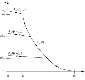
The function ![]() captures the general behavior to be expected in a ductile porous material. The unloaded virgin state corresponds to the value
captures the general behavior to be expected in a ductile porous material. The unloaded virgin state corresponds to the value ![]() , where
, where ![]() is the reference porosity of the material. Initial compression of the porous material is assumed to be elastic. Recall that decreasing porosity corresponds to a reduction in
is the reference porosity of the material. Initial compression of the porous material is assumed to be elastic. Recall that decreasing porosity corresponds to a reduction in ![]() . As the pressure increases beyond the elastic limit,
. As the pressure increases beyond the elastic limit, ![]() , the pores in the material start to crush, leading to irreversible compaction and permanent (plastic) volume change. Unloading from a partially compacted state follows a new elastic curve that depends on the maximum compaction (or, alternatively, the minimum value of
, the pores in the material start to crush, leading to irreversible compaction and permanent (plastic) volume change. Unloading from a partially compacted state follows a new elastic curve that depends on the maximum compaction (or, alternatively, the minimum value of ![]() ) ever attained during the deformation history of the material. The absolute value of the slope of the elastic curve decreases as
) ever attained during the deformation history of the material. The absolute value of the slope of the elastic curve decreases as ![]() decreases, as will be quantified later. The material becomes fully compacted when the pressure reaches the compaction pressure
decreases, as will be quantified later. The material becomes fully compacted when the pressure reaches the compaction pressure ![]() ; at that point
; at that point ![]() , a value that is retained forever. The function
, a value that is retained forever. The function ![]() therefore has multiple branches: a plastic branch,
therefore has multiple branches: a plastic branch, ![]() , and multiple elastic branches,
, and multiple elastic branches, ![]() , corresponding to elastic unloading from partially compacted states. The appropriate branch of A is selected according to the following rule:
, corresponding to elastic unloading from partially compacted states. The appropriate branch of A is selected according to the following rule:
![]()
![]()
![]()
![]()
If the solid phase is modeled using the Mie-Grüneisen equation of state, ![]() is given directly by the reference sound speed,
is given directly by the reference sound speed, ![]() . On the other hand, if the solid phase is modeled using the tabulated equation of state,
. On the other hand, if the solid phase is modeled using the tabulated equation of state, ![]() is computed from the initial bulk modulus and reference density of the solid material,
is computed from the initial bulk modulus and reference density of the solid material, ![]() . In this case the reference density is required to be constant; it cannot be a function of temperature or field variables.
. In this case the reference density is required to be constant; it cannot be a function of temperature or field variables.
Following Wardlaw et al. (1996), the above equation for the elastic curve in Abaqus/Explicit is simplified and replaced by the linear relations
![]()
| Input File Usage: | Use the following option to specify the reference density of the solid phase, |
*DENSITY Use one of the following options to specify additional material properties for the solid phase: *EOS, TYPE=USUP (if the solid phase is modeled using the Mie-Grüneisen equation of state) *EOS, TYPE=TABULAR (if the solid phase is modeled using the tabulated equation of state) Use the following option to specify the properties of the porous material (the reference sound speed, *EOS COMPACTION |
| Abaqus/CAE Usage: | Property module: material editor:
General |
Use one of the following options to specify additional material properties for the solid phase: Mechanical Use the following option to specify the properties of the porous material: Mechanical |
The initial state of the porous material is determined from the initial values of porosity, ![]() ; specific energy,
; specific energy, ![]() ; and pressure stress, p. Abaqus/Explicit automatically computes the initial density,
; and pressure stress, p. Abaqus/Explicit automatically computes the initial density, ![]() , that satisfies the equation of state,
, that satisfies the equation of state, ![]() . You can define the initial porosity, initial specific energy, and initial stress state (see “Initial conditions in Abaqus/Standard and Abaqus/Explicit,” Section 34.2.1). If no initial conditions are given, Abaqus/Explicit assumes that the material is at its virgin state:
. You can define the initial porosity, initial specific energy, and initial stress state (see “Initial conditions in Abaqus/Standard and Abaqus/Explicit,” Section 34.2.1). If no initial conditions are given, Abaqus/Explicit assumes that the material is at its virgin state:
Abaqus/Explicit will issue an error message if the initial ![]() state lies outside the region of allowed states (see Figure 25.2.1–2). When initial conditions are specified only for p (or for
state lies outside the region of allowed states (see Figure 25.2.1–2). When initial conditions are specified only for p (or for ![]() ), Abaqus/Explicit will compute
), Abaqus/Explicit will compute ![]() (or p) assuming that the
(or p) assuming that the ![]() state lies on the primary (monotonic loading) curve.
state lies on the primary (monotonic loading) curve.
| Input File Usage: | Use some or all of the following options, as required: |
*INITIAL CONDITIONS, TYPE=SPECIFIC ENERGY *INITIAL CONDITIONS, TYPE=STRESS *INITIAL CONDITIONS, TYPE=POROSITY |
| Abaqus/CAE Usage: | Load module: Create Predefined Field: Step: Initial: choose Mechanical for the Category and Stress for the Types for Selected Step |
Initial specific energy and initial porosity are not supported in Abaqus/CAE. |
The Jones-Wilkins-Lee (or JWL) equation of state models the pressure generated by the release of chemical energy in an explosive. This model is implemented in a form referred to as a programmed burn, which means that the reaction and initiation of the explosive is not determined by shock in the material. Instead, the initiation time is determined by a geometric construction using the detonation wave speed and the distance of the material point from the detonation points.
The JWL equation of state can be written in terms of the internal energy per unit mass, ![]() , as
, as
![]()
| Abaqus/CAE Usage: | Property module: material editor:
General |
Abaqus/Explicit calculates the arrival time of the detonation wave at a material point ![]() as the distance from the material point to the nearest detonation point divided by the detonation wave speed:
as the distance from the material point to the nearest detonation point divided by the detonation wave speed:
![]()
To spread the burn wave over several elements, a burn fraction, ![]() , is computed as
, is computed as
![]()
You can define any number of detonation points for the explosive material. Coordinates of the points must be defined along with a detonation delay time. Each material point responds to the first detonation point that it sees. The detonation arrival time at a material point is based upon the time that it takes a detonation wave (traveling at the detonation wave speed ![]() ) to reach the material point plus the detonation delay time for the detonation point. If there are multiple detonation points, the arrival time is based on the minimum arrival time for all the detonation points. In a body with curved surfaces care should be taken that the detonation arrival times are meaningful. The detonation arrival times are based on the straight line of sight from the material point to the detonation point. In a curved body the line of sight may pass outside of the body.
) to reach the material point plus the detonation delay time for the detonation point. If there are multiple detonation points, the arrival time is based on the minimum arrival time for all the detonation points. In a body with curved surfaces care should be taken that the detonation arrival times are meaningful. The detonation arrival times are based on the straight line of sight from the material point to the detonation point. In a curved body the line of sight may pass outside of the body.
| Input File Usage: | Use both of the following options to define the detonation points: |
*EOS, TYPE=JWL *DETONATION POINT |
| Abaqus/CAE Usage: | Property module: material editor: Mechanical |
Explosive materials generally have some nominal volumetric stiffness before detonation. It may be useful to incorporate this stiffness when elements modeled with a JWL equation of state are subjected to stress before initiation of detonation by the arriving detonation wave. You can define the pre-detonation bulk modulus, ![]() . The pressure will be computed from the volumetric strain and
. The pressure will be computed from the volumetric strain and ![]() until detonation, at which time the pressure will be determined by the procedure outlined above. The initial relative density (
until detonation, at which time the pressure will be determined by the procedure outlined above. The initial relative density (![]() ) used in the JWL equation is assumed to be unity. The initial specific energy
) used in the JWL equation is assumed to be unity. The initial specific energy ![]() is assumed to be equal to the user-defined detonation energy
is assumed to be equal to the user-defined detonation energy ![]() .
.
If you specify a nonzero value of ![]() , you can also define an initial stress state for the explosive materials.
, you can also define an initial stress state for the explosive materials.
| Input File Usage: | Use the following option to define the initial stress: |
*INITIAL CONDITIONS, TYPE=STRESS Optionally, you can also define the initial specific energy directly: *INITIAL CONDITIONS, TYPE=SPECIFIC ENERGY |
| Abaqus/CAE Usage: | Load module: Create Predefined Field: Step: Initial: choose Mechanical for the Category and Stress for the Types for Selected Step |
Initial specific energy is not supported in Abaqus/CAE. |
The ignition and growth equation of state models shock initiation and detonation wave propagation of solid high explosives. The heterogeneous explosive is modeled as a homogeneous mixture of two phases: the unreacted solid explosive and the reacted gas products. Separate JWL equations of state are prescribed for each phase:
![]()
![]()
![]()
![]()
| Abaqus/CAE Usage: | Property module: material editor:
General |
The mixture of unreacted solid explosive and reacted gas products is defined by the mass fraction
![]()
![]()
![]()
![]()
![]()
![]()
| Input File Usage: | Use the following options to define the specific heat of the unreacted solid explosive: |
*EOS, TYPE=IGNITION AND GROWTH
*SPECIFIC HEAT, DEPENDENCIES=n
Use the following options to define the specific heat of the reacted gas product: *EOS, TYPE=IGNITION AND GROWTH *GAS SPECIFIC HEAT, DEPENDENCIES=n |
| Abaqus/CAE Usage: | Use the following options to define the specific heat of the unreacted solid explosive: |
Property module: material editor:
Mechanical Use the following options to define the specific heat of the reacted gas product: Property module: material editor:
Mechanical You can toggle on Use temperature-dependent data to define the specific heat as a function of temperature and/or select the Number of field variables to define the specific heat as a function of field variables. |
The conversion of unreacted solid explosive to reacted gas products is governed by the reaction rate. The reaction rate equation in the ignition and growth model is a pressure-driven rule, which includes three terms:
![]()
The first term, ![]() , describes hot spot ignition by igniting some of the material relatively quickly but limiting it to a small proportion of the total solid
, describes hot spot ignition by igniting some of the material relatively quickly but limiting it to a small proportion of the total solid ![]() . The second term,
. The second term, ![]() , represents the growth of reaction from the hot spot sites into the material and describes the inward and outward grain burning phenomena; this term is limited to a proportion of the total solid
, represents the growth of reaction from the hot spot sites into the material and describes the inward and outward grain burning phenomena; this term is limited to a proportion of the total solid ![]() . The third term,
. The third term, ![]() , is used to describe the rapid transition to detonation observed in some energetic materials.
, is used to describe the rapid transition to detonation observed in some energetic materials.
| Input File Usage: | Use both of the following options to define the reaction rate: |
*EOS, TYPE=IGNITION AND GROWTH *REACTION RATE |
| Abaqus/CAE Usage: | Property module: material editor:
Mechanical |
The initial mass fraction of the unreacted solid explosive is assumed to be one. The initial relative density (![]() ) used in the ignition and growth equation is assumed to be unity. The initial specific energy can be defined for the unreacted explosive.
) used in the ignition and growth equation is assumed to be unity. The initial specific energy can be defined for the unreacted explosive.
| Input File Usage: | Use the following option to define the initial specific energy: |
*INITIAL CONDITIONS, TYPE=SPECIFIC ENERGY |
| Abaqus/CAE Usage: | Initial specific energy is not supported in Abaqus/CAE. |
An ideal gas equation of state can be written in the form of
![]()
One of the important features of an ideal gas is that its specific energy depends only upon its temperature; therefore, the specific energy can be integrated numerically as
![]()
Modeling with an ideal gas equation of state is typically performed adiabatically; the temperature increase is calculated directly at the material integration points according to the adiabatic thermal energy increase caused by the work ![]() , where v is the specific volume (the volume per unit mass,
, where v is the specific volume (the volume per unit mass, ![]() ). Therefore, unless a fully coupled temperature-displacement analysis is performed, an adiabatic condition is always assumed in Abaqus/Explicit.
). Therefore, unless a fully coupled temperature-displacement analysis is performed, an adiabatic condition is always assumed in Abaqus/Explicit.
When performing a fully coupled temperature-displacement analysis, the pressure stress and specific energy are updated based on the evolving temperature field. The energy increase due to the change in state will be accounted for in the heat equation and will be subject to heat conduction.
For the ideal gas model in Abaqus/Explicit you define the gas constant, R, and the ambient pressure, ![]() . For an ideal gas R can be determined from the universal gas constant,
. For an ideal gas R can be determined from the universal gas constant, ![]() , and the molecular weight,
, and the molecular weight, ![]() , as follows:
, as follows:
![]()
![]()
| Input File Usage: | Use both of the following options: |
*EOS, TYPE=IDEAL GAS *SPECIFIC HEAT, DEPENDENCIES=n |
| Abaqus/CAE Usage: | Property module: material editor:
Mechanical |
There are different methods to define the initial state of the gas. You can specify the initial density, ![]() , and either the initial pressure stress,
, and either the initial pressure stress, ![]() , or the initial temperature,
, or the initial temperature, ![]() . The initial value of the unspecified field (temperature or pressure) is determined from the equation of state. Alternatively, you can specify both the initial pressure stress and the initial temperature. In this case the user-specified initial density is replaced by that derived from the equation of state in terms of initial pressure and temperature.
. The initial value of the unspecified field (temperature or pressure) is determined from the equation of state. Alternatively, you can specify both the initial pressure stress and the initial temperature. In this case the user-specified initial density is replaced by that derived from the equation of state in terms of initial pressure and temperature.
By default, Abaqus/Explicit automatically computes the initial specific energy, ![]() , from the initial temperature by numerically integrating the equation
, from the initial temperature by numerically integrating the equation
![]()
| Input File Usage: | Use some or all of the following options, as required: |
*DENSITY, DEPENDENCIES=n
*INITIAL CONDITIONS, TYPE=STRESS
*INITIAL CONDITIONS, TYPE=TEMPERATURE
Use the following option to specify the initial specific energy directly: *INITIAL CONDITIONS, TYPE=SPECIFIC ENERGY |
| Abaqus/CAE Usage: | Property module: material editor: General |
Load module: Create Predefined Field: Step: Initial: choose Other for the Category and Temperature for the Types for Selected Step Load module: Create Predefined Field: Step: Initial: choose Mechanical for the Category and Stress for the Types for Selected Step Initial specific energy is not supported in Abaqus/CAE. |
When a non-absolute temperature scale is used, you must specify the value of absolute zero temperature.
| Input File Usage: | *PHYSICAL CONSTANTS, ABSOLUTE ZERO= |
| Abaqus/CAE Usage: | Any module: Model |
In the case of an adiabatic analysis with constant specific heat (both ![]() and
and ![]() are constant), the specific energy is linear in temperature
are constant), the specific energy is linear in temperature
![]()
![]()
![]()
![]()
for a monatomic;
![]()
for a diatomic; and
![]()
for a polyatomic gas.
The ideal gas equation of state can be used to model wave propagation effects and the dynamics of a spatially varying state of a gaseous region. For cases in which the inertial effects of the gas are not important and the state of the gas can be assumed to be uniform throughout a region, the hydrostatic fluid model (“Surface-based fluid cavities: overview,” Section 11.5.1) is a simpler, more computationally efficient alternative.
The equation of state defines only the material's hydrostatic behavior. It can be used by itself, in which case the material has only volumetric strength (the material is assumed to have no shear strength). Alternatively, Abaqus/Explicit allows you to define deviatoric behavior, assuming that the deviatoric and volumetric responses are uncoupled. Two models are available for the deviatoric response: a linear isotropic elastic model and a viscous model. The material's volumetric response is governed then by the equation of state model, while its deviatoric response is governed by either the linear isotropic elastic model or the viscous fluid model.
For the elastic shear behavior the deviatoric stress is related to the deviatoric strain as
![]()
| Abaqus/CAE Usage: | Property module: material editor: Mechanical |
For the viscous shear behavior the deviatoric stress is related to the deviatoric strain rate as
![]()
Abaqus/Explicit provides a wide range of viscosity models to describe both Newtonian and non-Newtonian fluids. These are described in “Viscosity,” Section 26.1.4.
| Input File Usage: | Use both of the following options to define viscous shear behavior: |
*EOS *VISCOSITY |
| Abaqus/CAE Usage: | Property module: material editor: Mechanical |
An equation of state model can be used with the Mises (“Classical metal plasticity,” Section 23.2.1) or the Johnson-Cook (“Johnson-Cook plasticity,” Section 23.2.7) plasticity models to model elastic-plastic behavior. In this case you must define the elastic part of the shear behavior. The material's volumetric response is governed by the equation of state model, while the deviatoric response is governed by the linear elastic shear and the plasticity model.
| Abaqus/CAE Usage: | Property module: material editor: |
You can specify initial conditions for the equivalent plastic strain, ![]() (“Initial conditions in Abaqus/Standard and Abaqus/Explicit,” Section 34.2.1).
(“Initial conditions in Abaqus/Standard and Abaqus/Explicit,” Section 34.2.1).
| Input File Usage: | *INITIAL CONDITIONS, TYPE=HARDENING |
| Abaqus/CAE Usage: | Load module: Create Predefined Field: Step: Initial, choose Mechanical for the Category and Hardening for the Types for Selected Step |
An equation of state model can be used in conjunction with the extended Drucker-Prager (“Extended Drucker-Prager models,” Section 23.3.1) plasticity models to model pressure-dependent plasticity behavior. This approach can be appropriate for modeling the response of ceramics and other brittle materials under high velocity impact conditions. In this case you must define the elastic part of the shear behavior. The material's deviatoric response is governed by the linear elastic shear and the pressure-dependent plasticity model, while the volumetric response is governed by the equation of state model. In particular, no plastic dilation effects are taken into account (if you specify a dilation angle other than zero, the value is ignored and Abaqus/Explicit issues a warning message).
“High-velocity impact of a ceramic target,” Section 2.1.18 of the Abaqus Example Problems Guide illustrates the use of an equation of state model with the extended Drucker-Prager plasticity models.
| Input File Usage: | Use the following options: |
*EOS *ELASTIC, TYPE=SHEAR *DRUCKER PRAGER *DRUCKER PRAGER HARDENING |
| Abaqus/CAE Usage: | Property module: material editor: |
You can specify initial conditions for the equivalent plastic strain, ![]() (“Initial conditions in Abaqus/Standard and Abaqus/Explicit,” Section 34.2.1).
(“Initial conditions in Abaqus/Standard and Abaqus/Explicit,” Section 34.2.1).
| Input File Usage: | *INITIAL CONDITIONS, TYPE=HARDENING |
| Abaqus/CAE Usage: | Load module: Create Predefined Field: Step: Initial, choose Mechanical for the Category and Hardening for the Types for Selected Step |
An equation of state model (except the ideal gas equation of state) can also be used with the tensile failure model (“Dynamic failure models,” Section 23.2.8) to model dynamic spall or a pressure cutoff. The tensile failure model uses the hydrostatic pressure stress as a failure measure and offers a number of failure choices. You must provide the hydrostatic cutoff stress.
You can specify that the deviatoric stresses should fail when the tensile failure criterion is met. In the case where the material's deviatoric behavior is not defined, this specification is meaningless and is, therefore, ignored.
The tensile failure model in Abaqus/Explicit is designed for high-strain-rate dynamic problems in which inertia effects are important. Therefore, it should be used only for such situations. Improper use of the tensile failure model may result in an incorrect simulation.
| Input File Usage: | Use the following options: |
*EOS *TENSILE FAILURE |
| Abaqus/CAE Usage: | The tensile failure model is not supported in Abaqus/CAE. |
An adiabatic condition is always assumed for materials modeled with an equation of state unless a dynamic coupled temperature-displacement procedure is used. The adiabatic condition is assumed irrespective of whether an adiabatic dynamic stress analysis step has been specified. The temperature increase is calculated directly at the material integration points according to the adiabatic thermal energy increase caused by the mechanical work
![]()
When performing a fully coupled temperature-displacement analysis, the specific energy is updated based on the evolving temperature field using
![]()
A linear ![]() equation of state model can be used to model incompressible viscous and inviscid laminar flow governed by the Navier-Stokes equation of motion. The volumetric response is governed by the equations of state, where the bulk modulus acts as a penalty parameter for the incompressible constraint.
equation of state model can be used to model incompressible viscous and inviscid laminar flow governed by the Navier-Stokes equation of motion. The volumetric response is governed by the equations of state, where the bulk modulus acts as a penalty parameter for the incompressible constraint.
To model a viscous laminar flow that follows the Navier-Poisson law of a Newtonian fluid, use the Newtonian viscous deviatoric model and define the viscosity as the real linear viscosity of the fluid. To model non-Newtonian viscous flow, use one of the nonlinear viscosity models available in Abaqus/Explicit. Appropriate initial conditions for velocity and stress are essential to get an accurate solution for this class of problems.
To model an incompressible inviscid fluid such as water in Abaqus/Explicit, it is useful to define a small amount of shear resistance to suppress shear modes that can otherwise tangle the mesh. Here the shear stiffness or shear viscosity acts as a penalty parameter. The shear modulus or viscosity should be small because flow is inviscid; a high shear modulus or viscosity will result in an overly stiff response. To avoid an overly stiff response, the internal forces arising due to the deviatoric response of the material should be kept several orders of magnitude below the forces arising due to the volumetric response. This can be done by choosing an elastic shear modulus that is several orders of magnitude lower than the bulk modulus. If the viscous model is used, the shear viscosity specified should be on the order of the shear modulus, calculated as above, scaled by the stable time increment. The expected stable time increment can be obtained from a data check analysis of the model. This method is a convenient way to approximate a shear resistance that will not introduce excessive viscosity in the material.
If a shear model is defined, the hourglass control forces are calculated based on the shear resistance of the material. Thus, in materials with extremely low or zero shear strengths such as inviscid fluids, the hourglass forces calculated based on the default parameters are insufficient to prevent spurious hourglass modes. Therefore, a sufficiently high hourglass scaling factor is recommended to increase the resistance to such modes.
Equations of state can be used with any solid (continuum) elements in Abaqus/Explicit except plane stress elements. For three-dimensional applications exhibiting high confinement, the default kinematic formulation is recommended with reduced-integration solid elements (see “Section controls,” Section 27.1.4).
In addition to the standard output identifiers available in Abaqus (“Abaqus/Explicit output variable identifiers,” Section 4.2.2), the following variables have special meaning for the equation of state models:
PALPH | Distension, |
PALPHMIN | Minimum value, |
PEEQ | Equivalent plastic strain, |
Carroll, M., and A. C. Holt, “Suggested Modification of the ![]() Model for Porous Materials,” Journal of Applied Physics, vol. 43, no.2, pp. 759–761, 1972.
Model for Porous Materials,” Journal of Applied Physics, vol. 43, no.2, pp. 759–761, 1972.
Dobratz, B. M., “LLNL Explosives Handbook, Properties of Chemical Explosives and Explosive Simulants,” UCRL-52997, Lawrence Livermore National Laboratory, Livermore, California, January 1981.
Herrmann, W., “Constitutive Equation for the Dynamic Compaction of Ductile Porous Materials,” Journal of Applied Physics, vol. 40, no.6, pp. 2490–2499, 1968.
Lee, E., M. Finger, and W. Collins, “JWL Equation of State Coefficients for High Explosives,” UCID-16189, Lawrence Livermore National Laboratory, Livermore, California, January 1973.
Wardlaw, A. B., R. McKeown, and H. Chen, “Implementation and Application of the ![]() Equation of State in the DYSMAS Code,” Naval Surface Warfare Center, Dahlgren Division, Report Number: NSWCDD/TR-95/107, May 1996.
Equation of State in the DYSMAS Code,” Naval Surface Warfare Center, Dahlgren Division, Report Number: NSWCDD/TR-95/107, May 1996.