Products: Abaqus/Explicit Abaqus/Viewer
A probability density function:
is used to define the statistical distributions of a continuous random variable; and
can be defined for uniform, normal, log-normal, piecewise linear, and discrete distributions.
There are many examples of randomness associated with data. Particle sizes in a granular media such as gravel are an example. Randomness observed in data can be described by statistical distributions. Pseudo-random numbers that are generated based on statistical distributions are used to capture randomness in data in a numerical simulation.
The size distribution of particle species generated by a particle generator can be described by statistical distributions.
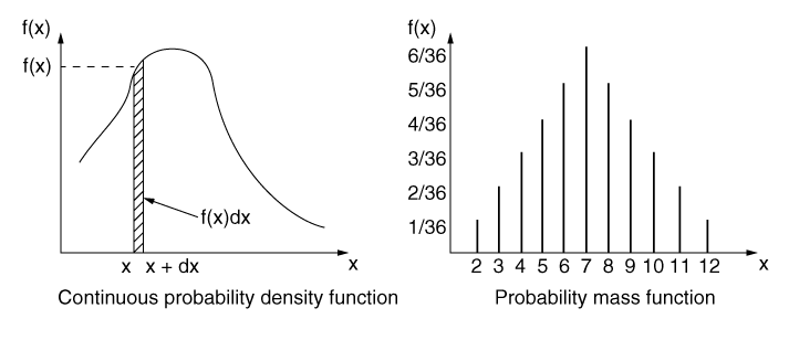
A probability density function (PDF) describes the probability of the value of a continuous random variable falling within a range. If the random variable can only have specific values (like throwing dice), a probability mass function (PMF) would be used to describe the probabilities of the outcomes. The plot on the left in Figure 2.12.1–1 shows a PDF for the random variable ![]() . The probability that the random variable has a value in the range
. The probability that the random variable has a value in the range ![]() and
and ![]() is
is ![]() . The probability that the random variable
. The probability that the random variable ![]() will be in the range
will be in the range ![]() is given by:
is given by:
![]()
![]()
The plot on the right in Figure 2.12.1–1 shows a PMF where the horizontal axis shows the specific values of the random variable and the vertical axis shows the corresponding probabilities.
Abaqus/Explicit supports uniform, normal (Gaussian), log-normal, piecewise linear, and discrete probability density functions. To define a probability density function, you must assign it a name and specify its type.
| Input File Usage: | *PROBABILITY DENSITY FUNCTION, NAME=PDF_name, TYPE=PDF_type |
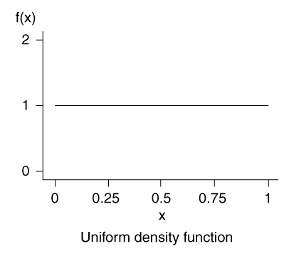
Uniform distributions (shown in Figure 2.12.1–2) have many applications, particularly in the numerical simulation of random processes. The following function describes a uniform probability density function for a random variable ![]() between
between ![]() and
and ![]() :
:
![]()
| Input File Usage: | *PROBABILITY DENSITY FUNCTION, TYPE=UNIFORM |
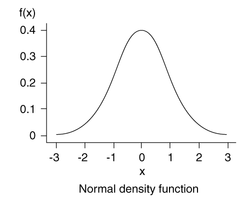
Normal distributions (shown in Figure 2.12.1–3) have many applications in science and engineering; for example, errors in experimental measurements are often assumed to have a normal distribution. The following function describes a normal probability density function:
| Input File Usage: | *PROBABILITY DENSITY FUNCTION, TYPE=NORMAL |
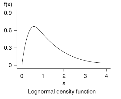
Log-normal distributions (shown in Figure 2.12.1–4) are used in describing many natural phenomena. They are commonly used to describe particle size distributions in soils. The following function describes a log-normal probability density function:
![]()
| Input File Usage: | *PROBABILITY DENSITY FUNCTION, TYPE=LOGNORMAL |
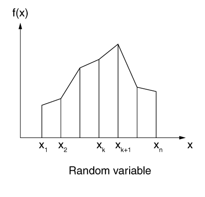
A piecewise linear probability density function can be used to approximate general distributions that are not well represented by the other PDF forms discussed above. With a piecewise linear probability density function, you specify PDF values at discrete points. Abaqus/Explicit considers linear variations in the PDF between these points, as shown in Figure 2.12.1–5. The PDF is zero below the first data point and above the last data point.
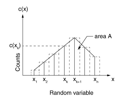
As mentioned earlier, the area under a PDF is unity. Abaqus/Explicit will renormalize the specified PDF data to achieve this requirement. This renormalization of data values allows you to specify relative PDF values that may be obtained from a histogram. A histogram contains the data in the form of a table of random variable ranges and the percentage or number that fall within those ranges. As shown in Figure 2.12.1–6, you specify a table of the midpoint value of each range in the histogram and the corresponding count:
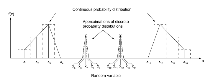
There may be situations where the random variable has continuous values over certain ranges and discrete values elsewhere. Figure 2.12.1–7 shows the use of a piecewise linear probability density function to approximate such distributions where the discrete values are approximated by continuous random variables spanning a very narrow range of values (for example, the discrete value ![]() is approximated by the continuous range from
is approximated by the continuous range from ![]() to
to ![]() ).
).
| Input File Usage: | *PROBABILITY DENSITY FUNCTION, TYPE=PIECEWISE LINEAR |
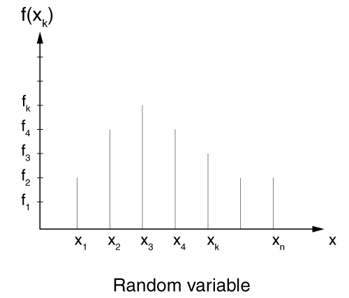
Some applications have only certain specific outcomes. These applications can be represented by a discrete probability density function, as shown in Figure 2.12.1–8. A simple example is throwing of a pair of dice. Only the outcomes of 2, 3, 4, 5, 6, 7, 8, 9, 10, 11, and 12 are possible, with the probabilities of 1/36, 2/36, 3/36, 4/36, 5/36, 6/36, 5/36, 4/36, 3/36, 2/36, and 1/36, respectively. A very specific case of a discrete probability density function is the case when only one value occurs with the probability of 1. To specify a discrete probability density function, you provide a table of the specific values of the random variable along with the corresponding probability:

| Input File Usage: | *PROBABILITY DENSITY FUNCTION, TYPE=DISCRETE |
The normal and log-normal probability density functions have open-ended characteristics. These PDFs can be truncated to enforce upper and lower bounds on the value of the random variable. Figure 2.12.1–9 shows a truncated normal distribution ![]() where all values of the random variable
where all values of the random variable ![]() and
and ![]() from the untruncated normal distribution
from the untruncated normal distribution ![]() have been rejected.
have been rejected.
![]()
You specify the lower and upper limits of the random variable along with the mean and standard deviation for these types of PDFs. The uniform and the piecewise linear distributions have lower and upper limits for the random variable built into the definition of the PDF and, therefore, do not require renormalization because of truncation.
Probability density functions are supported only for the size distributions of PD3D elements created using a particle generator.
The following example illustrates the use of a probability density function for particle size distribution:
*HEADING
…
*PARTICLE GENERATOR, NAME=generator_name, TYPE=PD3D,
MAXIMUM NUMBER OF PARTICLES=number
**
*PARTICLE GENERATOR INLET, SURFACE=inlet_surf
**
*PARTICLE GENERATOR MIXTURE
gen_SET1, gen_SET2
**
*PROBABILITY DENSITY FUNCTION, NAME=PDF_gen_SET1, TYPE=NORMAL
Data line to define PDF
*PROBABILITY DENSITY FUNCTION, NAME=PDF_gen_SET2, TYPE=LOGNORMAL
Data line to define PDF
**
*DISCRETE SECTION, ELSET=gen_SET1
PDF_gen_SET1
*DISCRETE SECTION, ELSET=gen_SET2
PDF_gen_SET2
…
*END STEP
Benjamin, J. R., and C. A. Cornell, “Probability, Statistics, and Decision for Civil Engineers,” McGraw-Hill, 1970.
Press, W. H., S. A. Teukolsky, W. T. Vetterling, and B. P. Flannery, “Numerical Recipes in Fortran 77, The Art of Scientific Computing,” University of Cambridge, 1992.
Saucier, R., “Computer Generation of Statistical Distributions,” Army Research Laboratory, 2000.