Product: Abaqus/Explicit

User subroutine VUANISOHYPER_INV:
can be used to define the strain energy potential of anisotropic hyperelastic materials as a function of an irreducible set of scalar invariants;
will be called for blocks of material calculation points for which the material definition contains user-defined anisotropic hyperelastic behavior with invariant-based formulation (“Anisotropic hyperelastic behavior,” Section 22.5.3 of the Abaqus Analysis User's Guide);
can use and update solution-dependent state variables;
can use any field variables that are passed in; and
requires that the values of the derivatives of the strain energy density function be defined with respect to the scalar invariants.
To facilitate coding and provide easy access to the array of invariants passed to user subroutine VUANISOHYPER_INV, an enumerated representation of each invariant is introduced. Any scalar invariant can, therefore, be represented uniquely by an enumerated invariant, ![]() , where the subscript n denotes the order of the invariant according to the enumeration scheme in the following table:
, where the subscript n denotes the order of the invariant according to the enumeration scheme in the following table:
For example, in the case of three families of fibers there are a total of 15 invariants: ![]() ,
, ![]() ,
, ![]() , six invariants of type
, six invariants of type ![]() , and six invariants of type
, and six invariants of type ![]() , with
, with ![]() . The following correspondence exists between each of these invariants and their enumerated counterpart:
. The following correspondence exists between each of these invariants and their enumerated counterpart:
A similar scheme is used for the array zeta of terms ![]() . Each term can be represented uniquely by an enumerated counterpart
. Each term can be represented uniquely by an enumerated counterpart ![]() , as shown below:
, as shown below:
The components of the array duDi of first derivatives of the strain energy potential with respect to the scalar invariants, ![]() , are stored using the enumeration scheme discussed above for the scalar invariants.
, are stored using the enumeration scheme discussed above for the scalar invariants.
The elements of the array d2uDiDi of second derivatives of the strain energy function, ![]() , are laid out in memory using triangular storage: if
, are laid out in memory using triangular storage: if ![]() denotes the component in this array corresponding to the term
denotes the component in this array corresponding to the term ![]() , then
, then ![]() . For example, the term
. For example, the term ![]() is stored in component
is stored in component ![]() in the d2uDiDi array.
in the d2uDiDi array.
When VUANISOHYPER_INV is used to define the material response of shell elements, Abaqus/Explicit cannot calculate a default value for the transverse shear stiffness of the element. Hence, you must define the element's transverse shear stiffness. See “Shell section behavior,” Section 29.6.4 of the Abaqus Analysis User's Guide, for guidelines on choosing this stiffness.
Material points that satisfy a user-defined failure criterion can be deleted from the model (see “User-defined mechanical material behavior,” Section 26.7.1 of the Abaqus Analysis User's Guide). You must specify the state variable number controlling the element deletion flag when you allocate space for the solution-dependent state variables, as explained in “User-defined mechanical material behavior,” Section 26.7.1 of the Abaqus Analysis User's Guide. The deletion state variable should be set to a value of one or zero in VUANISOHYPER_INV. A value of one indicates that the material point is active, and a value of zero indicates that Abaqus/Explicit should delete the material point from the model by setting the stresses to zero. The structure of the block of material points passed to user subroutine VUANISOHYPER_INV remains unchanged during the analysis; deleted material points are not removed from the block. Abaqus/Explicit will “freeze” the values of the invariants passed to VUANISOHYPER_INV for all deleted material points; that is, the values remain constant after deletion is triggered. Once a material point has been flagged as deleted, it cannot be reactivated.
      subroutine vuanisohyper_inv (
C Read only (unmodifiable) variables –
     1     nblock, nFiber, nInv,
     2     jElem, kIntPt, kLayer, kSecPt,
     3     cmname,
     4     nstatev, nfieldv, nprops,
     5     props, tempOld, tempNew, fieldOld, fieldNew,
     6     stateOld, sInvariant, zeta,
C Write only (modifiable) variables –
     7     uDev, duDi, d2uDiDi,
     8     stateNew )
C
      include 'vaba_param.inc'
C
      dimension props(nprops),
     1  tempOld(nblock),
     2  fieldOld(nblock,nfieldv),
     3  stateOld(nblock,nstatev),
     4  tempNew(nblock),
     5  fieldNew(nblock,nfieldv),
     6  sInvariant(nblock,nInv),
     7  zeta(nblock,nFiber*(nFiber-1)/2),
     8  uDev(nblock), duDi(nblock,nInv),
     9  d2uDiDi(nblock,nInv*(nInv+1)/2),
     *  stateNew(nblock,nstatev)
C
      character*80 cmname
C

      do 100 km = 1,nblock
        user coding
  100 continue

      return
endudev(nblock)
![]() , the deviatoric part of the strain energy density of the primary material response. This quantity is needed only if the current material definition also includes Mullins effect (see “Mullins effect,” Section 22.6.1 of the Abaqus Analysis User's Guide).
, the deviatoric part of the strain energy density of the primary material response. This quantity is needed only if the current material definition also includes Mullins effect (see “Mullins effect,” Section 22.6.1 of the Abaqus Analysis User's Guide).
duDi(nblock,nInv)
Array of derivatives of strain energy potential with respect to the scalar invariants, ![]() , ordered using the enumeration scheme discussed above.
, ordered using the enumeration scheme discussed above.
d2uDiDi(nblock,nInv*(nInv+1)/2)
Arrays of second derivatives of strain energy potential with respect to the scalar invariants (using triangular storage), ![]() .
.
stateNew(nblock,nstatev)
State variables at each material point at the end of the increment. You define the size of this array by allocating space for it (see “User subroutines: overview,” Section 18.1.1 of the Abaqus Analysis User's Guide, for more information).
nblock
Number of material points to be processed in this call to VUANISOHYPER_STRAIN.
nFiber
Number of families of fibers defined for this material.
nInv
Number of scalar invariants.
jElem(nblock)
Array of element numbers.
kIntPt
Integration point number.
kLayer
Layer number (for composite shells).
kSecPt
Section point number within the current layer.
cmname
User-specified material name, left justified. It is passed in as an uppercase character string. Some internal material models are given names starting with the “ABQ_” character string. To avoid conflict, you should not use “ABQ_” as the leading string for cmname.
nstatev
Number of user-defined state variables that are associated with this material type (you define this as described in “Allocating space” in “User subroutines: overview,” Section 18.1.1 of the Abaqus Analysis User's Guide).
nfieldv
Number of user-defined external field variables.
nprops
User-specified number of user-defined material properties.
props(nprops)
User-supplied material properties.
tempOld(nblock)
Temperatures at each material point at the beginning of the increment.
tempNew(nblock)
Temperatures at each material point at the end of the increment.
fieldOld(nblock,nfieldv)
Values of the user-defined field variables at each material point at the beginning of the increment.
fieldNew(nblock,nfieldv)
Values of the user-defined field variables at each material point at the end of the increment.
stateOld(nblock,nstatev)
State variables at each material point at the beginning of the increment.
sInvariant(nblock,nInv)
Array of scalar invariants,![]() , at each material point at the end of the increment. The invariants are ordered using the enumeration scheme discussed above.
, at each material point at the end of the increment. The invariants are ordered using the enumeration scheme discussed above.
zeta(nblock,nFiber*(nFiber-1)/2) )
Array of dot product between the directions of different families of fiber in the reference configuration, ![]() . The array contains the enumerated values
. The array contains the enumerated values ![]() using the scheme discussed above.
using the scheme discussed above.
To use more than one user-defined anisotropic hyperelastic material model, the variable cmname can be tested for different material names inside user subroutine VUANISOHYPER_INV, as illustrated below:
if (cmname(1:4) .eq. 'MAT1') then
   call VUANISOHYPER_INV1(argument_list)
else if (cmname(1:4) .eq. 'MAT2') then
   call VUANISOHYPER_INV2(argument_list)
end if
VUANISOHYPER_INV1 and VUANISOHYPER_INV2 are the actual subroutines containing the anisotropic hyperelastic models for each material MAT1 and MAT2, respectively. Subroutine VUANISOHYPER_INV merely acts as a directory here. The argument list can be the same as that used in subroutine VUANISOHYPER_INV. The material names must be in uppercase characters since cmname is passed in as an uppercase character string.
As an example of the coding of subroutine VUANISOHYPER_INV, consider the model proposed by Kaliske and Schmidt (2005) for nonlinear anisotropic elasticity with two families of fibers. The strain energy function is given by a polynomial series expansion in the form
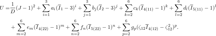
The code in subroutine VUANISOHYPER_INV must return the derivatives of the strain energy function with respect to the scalar invariants, which are readily computed from the above expression. In this example auxiliary functions are used to facilitate enumeration of pseudo-invarinats of type ![]() and
and ![]() , as well as for indexing into the array of second derivatives using symmetric storage. The subroutine would be coded as follows:
, as well as for indexing into the array of second derivatives using symmetric storage. The subroutine would be coded as follows:
      subroutine vuanisohyper_inv (
C Read only -
     *     nblock, nFiber, nInv,
     *     jElem, kIntPt, kLayer, kSecPt,
     *     cmname,
     *     nstatev, nfieldv, nprops,
     *     props, tempOld, tempNew, fieldOld, fieldNew,
     *     stateOld, sInvariant, zeta,
C     Write only -
     *     uDev, duDi, d2uDiDi,
     *     stateNew )
C
      include 'vaba_param.inc'
C
      dimension props(nprops),
     *  tempOld(nblock),
     *  fieldOld(nblock,nfieldv),
     *  stateOld(nblock,nstatev),
     *  tempNew(nblock),
     *  fieldNew(nblock,nfieldv),
     *  sInvariant(nblock,nInv),
     *  zeta(nblock,nFiber*(nFiber-1)/2),
     *  uDev(nblock), duDi(nblock,*),
     *  d2uDiDi(nblock,*),
     *  stateNew(nblock,nstatev)
C
      character*80 cmname
C
      parameter ( zero = 0.d0, one = 1.d0, two = 2.d0,
     *     three = 3.d0, four = 4.d0, five = 5.d0, six = 6.d0 )
C
C     Kaliske energy function (3D)
C
C     Read material properties
      d=props(1)
      dinv = one / d
      a1=props(2)
      a2=props(3)
      a3=props(4)
      b1=props(5)
      b2=props(6)
      b3=props(7)
      c2=props(8)
      c3=props(9)
      c4=props(10)
      c5=props(11)
      c6=props(12)
      d2=props(13)
      d3=props(14)
      d4=props(15)
      d5=props(16)
      d6=props(17)
      e2=props(18)
      e3=props(19)
      e4=props(20)
      e5=props(21)
      e6=props(22)
      f2=props(23)
      f3=props(24)
      f4=props(25)
      f5=props(26)
      f6=props(27)
      g2=props(28)
      g3=props(29)
      g4=props(30)
      g5=props(31)
      g6=props(32)
C
      do k = 1, nblock
         Udev(k) = zero
C     Compute Udev and 1st and 2nd derivatives w.r.t invariants
C     - I1
         bi1 = sInvariant(k,1)
         term = bi1-three
         Udev(k) = Udev(k)
     *        + a1*term + a2*term**2 + a3*term**3
         duDi(k,1) = a1 + two*a2*term + three*a3*term**2
         d2uDiDi(k,indx(1,1)) = two*a2 + three*two*a3*term
C     - I2
         bi2 = sInvariant(k,2)
         term = bi2-three
         Udev(k) = Udev(k)
     *        + b1*term + b2*term**2 + b3*term**3
         duDi(k,2) = b1 + two*b2*term + three*b3*term**2
         d2uDiDi(k,indx(2,2)) = two*b2 + three*two*b3*term
C     - I3 (=J)
         bi3 = sInvariant(k,3)
         term = bi3-one
         duDi(k,3) = two*dinv*term
         d2uDiDi(k,indx(3,3)) = two*dinv
C     - I4(11)
         nI411 = indxInv4(1,1)
         bi411 = sInvariant(k,nI411)
         term = bi411-one
         Udev(k) = Udev(k)
     *        + c2*term**2 + c3*term**3 + c4*term**4
     *        + c5*term**5 + c6*term**6
         duDi(k,nI411) =
     *          two*c2*term
     *        + three*c3*term**2
     *        + four*c4*term**3
     *        + five*c5*term**4
     *        + six*c6*term**5
         d2uDiDi(k,indx(nI411,nI411)) =
     *          two*c2
     *        + three*two*c3*term
     *        + four*three*c4*term**2
     *        + five*four*c5*term**3
     *        + six*five*c6*term**4
C     - I5(11)
         nI511 = indxInv5(1,1)
         bi511 = sInvariant(k,nI511)
         term = bi511-one
         Udev(k) = Udev(k)
     *        + d2*term**2 + d3*term**3 + d4*term**4
     *        + d5*term**5 + d6*term**6
         duDi(k,nI511) =
     *          two*d2*term
     *        + three*d3*term**2
     *        + four*d4*term**3
     *        + five*d5*term**4
     *        + six*d6*term**5
         d2uDiDi(k,indx(nI511,nI511)) =
     *          two*d2
     *        + three*two*d3*term
     *        + four*three*d4*term**2
     *        + five*four*d5*term**3
     *        + six*five*d6*term**4
C     - I4(22)
         nI422 = indxInv4(2,2)
         bi422 = sInvariant(k,nI422)
         term = bi422-one
         Udev(k) = Udev(k)
     *        + e2*term**2 + e3*term**3 + e4*term**4
     *        + e5*term**5 + e6*term**6
         duDi(k,nI422) =
     *          two*e2*term
     *        + three*e3*term**2
     *        + four*e4*term**3
     *        + five*e5*term**4
     *        + six*e6*term**5
         d2uDiDi(k,indx(nI422,nI422)) =
     *          two*e2
     *        + three*two*e3*term
     *        + four*three*e4*term**2
     *        + five*four*e5*term**3
     *        + six*five*e6*term**4
C     - I5(22)
         nI522 = indxInv5(2,2)
         bi522 = sInvariant(k,nI522)
         term = bi522-one
         Udev(k) = Udev(k)
     *        + f2*term**2 + f3*term**3 + f4*term**4
     *        + f5*term**5 + f6*term**6
         duDi(k,nI522) =
     *          two*f2*term
     *        + three*f3*term**2
     *        + four*f4*term**3
     *        + five*f5*term**4
     *        + six*f6*term**5
         d2uDiDi(k,indx(nI522,nI522)) =
     *          two*f2
     *        + three*two*f3*term
     *        + four*three*f4*term**2
     *        + five*four*f5*term**3
     *        + six*five*f6*term**4
C     - I4(12)
         nI412 = indxInv4(1,2)
         bi412 = sInvariant(k,nI412)
         term = zeta(k,1)*(bi412-zeta(k,1))
         Udev(k) = Udev(k)
     *        + g2*term**2 + g3*term**3
     *        + g4*term**4 + g5*term**5
     *        + g6*term**6
         duDi(k,nI412) = zeta(k,1) * (
     *          two*g2*term
     *        + three*g3*term**2
     *        + four*g4*term**3
     *        + five*g5*term**4
     *        + six*g6*term**5 )
         d2uDiDi(k,indx(nI412,nI412)) = zeta(k,1)**2 * (
     *          two*g2
     *        + three*two*g3*term
     *        + four*three*g4*term**2
     *        + five*four*g5*term**3
     *        + six*five*g6*term**4 )
C
      end do
C
      return
      end
C
C     Function to map index from Square to Triangular storage
C     of symmetric matrix
C
      integer function indx( i, j )
      include 'vaba_param.inc'
      ii = min(i,j)
      jj = max(i,j)
      indx = ii + jj*(jj-1)/2
      return
      end
C
C     Function to generate enumeration of scalar
C     Pseudo-Invariants of type 4

C     integer function indxInv4( i, j )
      include 'vaba_param.inc'
      ii = min(i,j)
      jj = max(i,j)
      indxInv4 = 4 + jj*(jj-1) + 2*(ii-1)
      return
      end
C
C     Function to generate enumeration of scalar
C     Pseudo-Invariants of type 5
C
      integer function indxInv5( i, j )
      include 'vaba_param.inc'
      ii = min(i,j)
      jj = max(i,j)
      indxInv5 = 5 + jj*(jj-1) + 2*(ii-1)
      return
      end