Product: Abaqus/Standard
The modal dynamic procedure provides time history analysis of linear systems.
The excitation is given as a function of time: it is assumed that the amplitude curve is specified so that the magnitude of the excitation varies linearly within each increment. When the model is projected onto the eigenmodes used for its dynamic representation, we obtain the following set of equations at time t:
where theIf the projected damping matrix is diagonal, Equation 2.5.5–1 becomes the following uncoupled set of equations:
where![]()

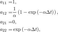
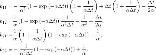
The solution to the uncoupled equations is obtained readily as a particular integral for the loading and a solution to the homogeneous equation (with no right-hand side). These solutions can be combined and written in the general form
whereThere are three cases of this solution for nonrigid body motion (![]() ), depending on whether the damping in the modal equilibrium equation is greater than, equal to, or less than critical damping (that is, depending on whether
), depending on whether the damping in the modal equilibrium equation is greater than, equal to, or less than critical damping (that is, depending on whether ![]() is positive, zero, or negative).
is positive, zero, or negative).

Equation 2.5.5–3 can be generalized to address full coupling in the projected damping matrix. Let the matrix ![]() be split into its diagonal and off-diagonal parts so that
be split into its diagonal and off-diagonal parts so that
![]()
![]()

There are three cases of this solution for nonrigid body motion (![]() ), depending on whether the damping in the modal equilibrium equation is greater than, equal to, or less than critical damping (that is, depending on whether
), depending on whether the damping in the modal equilibrium equation is greater than, equal to, or less than critical damping (that is, depending on whether ![]() is positive, zero, or negative).
is positive, zero, or negative).
If there are rigid body modes in the finite element model, there will be one or several eigenvalues that are zero. The equation of motion (Equation 2.5.5–1) is reduced to
Only Rayleigh damping can be specified for a rigid body mode, since the critical damping is zero. Furthermore, since it is a rigid body mode, only the mass damping factor, ![]() , appears (stiffness damping requires that there be straining of the body). For this case
, appears (stiffness damping requires that there be straining of the body). For this case


For the particular case of a rigid body mode without damping, the equation of motion (Equation 2.5.5–1) is reduced to
For this case

Structural damping is a commonly used damping model that represents damping as complex stiffness. This representation causes no difficulty for frequency domain analysis such as steady-state dynamics for which the solution is already complex. However, in the time domain, the solution must remain real-valued. To allow users to apply their structural damping model in the time domain, a method has been developed to convert structural damping to an equivalent viscous damping. This technique was designed so that, in the frequency domain, the viscous damping applied is identical to structural damping if the projected damping matrix is diagonal.
We start with the equation of a single degree-of-freedom oscillator,
![]()
![]()
Based on the two previous equations, if we want the viscous damping factor to have the same effect as the structural damping factor, we must have
![]()
![]()
![]()
![]()
![]()
![]()
![]()
![]()

The time integration is done in terms of the generalized coordinates, and the response of the physical variables is then immediately available by summation:
![]()
![]()
![]()
![]()

At the beginning of the step initial displacements and initial velocities must be converted to equivalent values of the generalized coordinates, which can be done exactly only if the number of eigenvectors equals the number of degrees of freedom. Since this is usually not the case, the initial values of the generalized coordinate displacement and velocity are calculated as
![]()
Similarly, for the initial velocities
![]()
For the case where the initial conditions are given by a previous modal dynamic analysis, the generalized displacement, velocity, and acceleration are simply taken from the previous analysis.

Many linear dynamic problems involve finding the response of a structure to a “base motion”: a time history of displacement, velocity, or acceleration given for the points where the displacements of the structure are prescribed. In all cases these base motions are converted into an acceleration history. If the displacement or velocity history has nonzero values at time ![]() 0, corrections to the acceleration histories are made at times
0, corrections to the acceleration histories are made at times ![]() 0 and
0 and ![]() . If velocities are given, the acceleration at
. If velocities are given, the acceleration at ![]() 0 is
0 is
![]()
![]()
If velocities are given for tabular or equally spaced amplitude curve definitions, the acceleration is defined by the central difference rule
![]()
![]()
The response is calculated relative to the base. If total values of nodal variables are required, the motion at the base is added to the relative values:

